[1]:
import numpy as np
import fermifab
from scipy.special import binom
1. What is FermiFab?
FermiFab stands for “fermion laboratory” and is a quantum physics toolbox for small numbers of fermions. It is mainly concerned with the representation of (symbolic) fermionic wavefunctions and the calculation of their reduced density matrices (RDMs). The toolbox transparently handles the inherent antisymmetrization of wavefunctions and incorporates the creation and annihilation formalism.
FermiFab is available at https://github.com/cmendl/fermifab.
2. Fermi states
A fundamental building block of multi-fermion quantum mechanics are Slater determinants, which you can think of as a collection of “orbitals” (or slots), some of which are occupied by a fermionic particle (e.g., an electron):
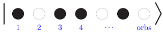
In this illustration, each circle represents an orbital, and the filled circles denote occupied orbitals. In mathematical terms, the available number of orbitals ‘orbs’ is the dimension of the underlying single-particle Hilbert space \(\mathcal{H}\) and the number of occupied orbitals is the particle number \(N\). Thus there are altogether
Slater determinants. Each quantum mechanical Fermi state is a linear combination of these Slater determinants with complex coefficients. Formally, the quantum Fermi state is an element of the \(N\)-particle Fock space \(\wedge^N \mathcal{H}\).
In FermiFab, you can define, say, a \(N=4\) particle state (or wavefunction) \(\psi\) and 6 available orbitals with the FermiState command:
[2]:
orbs = 6
N = 4
x = np.zeros(int(binom(orbs, N)), dtype=complex)
x[0] = 1/np.sqrt(2)
x[1] = 1j/np.sqrt(2)
psi = fermifab.FermiState(orbs, N, x)
psi
[2]:
Fermi State (orbs == 6, N == 4)

Vector representation w.r.t. ordered Slater basis:

array([0.70710678+0.j        , 0.        +0.70710678j,
       0.        +0.j        , 0.        +0.j        ,
       0.        +0.j        , 0.        +0.j        ,
       0.        +0.j        , 0.        +0.j        ,
       0.        +0.j        , 0.        +0.j        ,
       0.        +0.j        , 0.        +0.j        ,
       0.        +0.j        , 0.        +0.j        ,
       0.        +0.j        ])
The vector \(x\) contains the Slater determinant coefficients of \(\psi\) in lexicographical order.
The rank-one projector in bra-ket notation, \(|\psi\rangle\langle\psi|\), or “density matrix” of \(\psi\) can be calculated intuitively by
[3]:
psi @ psi.H
[3]:
Fermi Operator wedge^4 H -> wedge^4 H (orbs == 6)

Matrix representation w.r.t. ordered Slater basis:

array([[0.5+0.j , 0. -0.5j, 0. +0.j , 0. +0.j , 0. +0.j , 0. +0.j ,
        0. +0.j , 0. +0.j , 0. +0.j , 0. +0.j , 0. +0.j , 0. +0.j ,
        0. +0.j , 0. +0.j , 0. +0.j ],
       [0. +0.5j, 0.5+0.j , 0. +0.j , 0. +0.j , 0. +0.j , 0. +0.j ,
        0. +0.j , 0. +0.j , 0. +0.j , 0. +0.j , 0. +0.j , 0. +0.j ,
        0. +0.j , 0. +0.j , 0. +0.j ],
       [0. +0.j , 0. +0.j , 0. +0.j , 0. +0.j , 0. +0.j , 0. +0.j ,
        0. +0.j , 0. +0.j , 0. +0.j , 0. +0.j , 0. +0.j , 0. +0.j ,
        0. +0.j , 0. +0.j , 0. +0.j ],
       [0. +0.j , 0. +0.j , 0. +0.j , 0. +0.j , 0. +0.j , 0. +0.j ,
        0. +0.j , 0. +0.j , 0. +0.j , 0. +0.j , 0. +0.j , 0. +0.j ,
        0. +0.j , 0. +0.j , 0. +0.j ],
       [0. +0.j , 0. +0.j , 0. +0.j , 0. +0.j , 0. +0.j , 0. +0.j ,
        0. +0.j , 0. +0.j , 0. +0.j , 0. +0.j , 0. +0.j , 0. +0.j ,
        0. +0.j , 0. +0.j , 0. +0.j ],
       [0. +0.j , 0. +0.j , 0. +0.j , 0. +0.j , 0. +0.j , 0. +0.j ,
        0. +0.j , 0. +0.j , 0. +0.j , 0. +0.j , 0. +0.j , 0. +0.j ,
        0. +0.j , 0. +0.j , 0. +0.j ],
       [0. +0.j , 0. +0.j , 0. +0.j , 0. +0.j , 0. +0.j , 0. +0.j ,
        0. +0.j , 0. +0.j , 0. +0.j , 0. +0.j , 0. +0.j , 0. +0.j ,
        0. +0.j , 0. +0.j , 0. +0.j ],
       [0. +0.j , 0. +0.j , 0. +0.j , 0. +0.j , 0. +0.j , 0. +0.j ,
        0. +0.j , 0. +0.j , 0. +0.j , 0. +0.j , 0. +0.j , 0. +0.j ,
        0. +0.j , 0. +0.j , 0. +0.j ],
       [0. +0.j , 0. +0.j , 0. +0.j , 0. +0.j , 0. +0.j , 0. +0.j ,
        0. +0.j , 0. +0.j , 0. +0.j , 0. +0.j , 0. +0.j , 0. +0.j ,
        0. +0.j , 0. +0.j , 0. +0.j ],
       [0. +0.j , 0. +0.j , 0. +0.j , 0. +0.j , 0. +0.j , 0. +0.j ,
        0. +0.j , 0. +0.j , 0. +0.j , 0. +0.j , 0. +0.j , 0. +0.j ,
        0. +0.j , 0. +0.j , 0. +0.j ],
       [0. +0.j , 0. +0.j , 0. +0.j , 0. +0.j , 0. +0.j , 0. +0.j ,
        0. +0.j , 0. +0.j , 0. +0.j , 0. +0.j , 0. +0.j , 0. +0.j ,
        0. +0.j , 0. +0.j , 0. +0.j ],
       [0. +0.j , 0. +0.j , 0. +0.j , 0. +0.j , 0. +0.j , 0. +0.j ,
        0. +0.j , 0. +0.j , 0. +0.j , 0. +0.j , 0. +0.j , 0. +0.j ,
        0. +0.j , 0. +0.j , 0. +0.j ],
       [0. +0.j , 0. +0.j , 0. +0.j , 0. +0.j , 0. +0.j , 0. +0.j ,
        0. +0.j , 0. +0.j , 0. +0.j , 0. +0.j , 0. +0.j , 0. +0.j ,
        0. +0.j , 0. +0.j , 0. +0.j ],
       [0. +0.j , 0. +0.j , 0. +0.j , 0. +0.j , 0. +0.j , 0. +0.j ,
        0. +0.j , 0. +0.j , 0. +0.j , 0. +0.j , 0. +0.j , 0. +0.j ,
        0. +0.j , 0. +0.j , 0. +0.j ],
       [0. +0.j , 0. +0.j , 0. +0.j , 0. +0.j , 0. +0.j , 0. +0.j ,
        0. +0.j , 0. +0.j , 0. +0.j , 0. +0.j , 0. +0.j , 0. +0.j ,
        0. +0.j , 0. +0.j , 0. +0.j ]])
Note that the result is now an operator acting on the 4-particle antisymmetrized Hilbert space \(\wedge^4 \mathcal{H}\) !
3. Reduced density matrices (RDMs)
The core feature of the toolbox is the efficient calculation of reduced density matrices. For example, the two-body reduced density matrix \(\Gamma_\psi\) defined by
can be calculated by the rdm command as
[4]:
fermifab.rdm(psi, 2)
[4]:
Fermi Operator wedge^2 H -> wedge^2 H (orbs == 6)

Matrix representation w.r.t. ordered Slater basis:

array([[1. +0.j , 0. +0.j , 0. +0.j , 0. +0.j , 0. +0.j , 0. +0.j ,
        0. +0.j , 0. +0.j , 0. +0.j , 0. +0.j , 0. +0.j , 0. +0.j ,
        0. +0.j , 0. +0.j , 0. +0.j ],
       [0. +0.j , 1. +0.j , 0. +0.j , 0. +0.j , 0. +0.j , 0. +0.j ,
        0. +0.j , 0. +0.j , 0. +0.j , 0. +0.j , 0. +0.j , 0. +0.j ,
        0. +0.j , 0. +0.j , 0. +0.j ],
       [0. +0.j , 0. +0.j , 1. +0.j , 0. +0.j , 0. +0.j , 0. +0.j ,
        0. +0.j , 0. +0.j , 0. +0.j , 0. +0.j , 0. +0.j , 0. +0.j ,
        0. +0.j , 0. +0.j , 0. +0.j ],
       [0. +0.j , 0. +0.j , 0. +0.j , 0.5+0.j , 0. +0.j , 0. +0.j ,
        0. -0.5j, 0. +0.j , 0. +0.j , 0. +0.j , 0. +0.j , 0. +0.j ,
        0. +0.j , 0. +0.j , 0. +0.j ],
       [0. +0.j , 0. +0.j , 0. +0.j , 0. +0.j , 0.5+0.j , 0. +0.j ,
        0. +0.j , 0. -0.5j, 0. +0.j , 0. +0.j , 0. +0.j , 0. +0.j ,
        0. +0.j , 0. +0.j , 0. +0.j ],
       [0. +0.j , 0. +0.j , 0. +0.j , 0. +0.j , 0. +0.j , 0.5+0.j ,
        0. +0.j , 0. +0.j , 0. -0.5j, 0. +0.j , 0. +0.j , 0. +0.j ,
        0. +0.j , 0. +0.j , 0. +0.j ],
       [0. +0.j , 0. +0.j , 0. +0.j , 0. +0.5j, 0. +0.j , 0. +0.j ,
        0.5+0.j , 0. +0.j , 0. +0.j , 0. +0.j , 0. +0.j , 0. +0.j ,
        0. +0.j , 0. +0.j , 0. +0.j ],
       [0. +0.j , 0. +0.j , 0. +0.j , 0. +0.j , 0. +0.5j, 0. +0.j ,
        0. +0.j , 0.5+0.j , 0. +0.j , 0. +0.j , 0. +0.j , 0. +0.j ,
        0. +0.j , 0. +0.j , 0. +0.j ],
       [0. +0.j , 0. +0.j , 0. +0.j , 0. +0.j , 0. +0.j , 0. +0.5j,
        0. +0.j , 0. +0.j , 0.5+0.j , 0. +0.j , 0. +0.j , 0. +0.j ,
        0. +0.j , 0. +0.j , 0. +0.j ],
       [0. +0.j , 0. +0.j , 0. +0.j , 0. +0.j , 0. +0.j , 0. +0.j ,
        0. +0.j , 0. +0.j , 0. +0.j , 0. +0.j , 0. +0.j , 0. +0.j ,
        0. +0.j , 0. +0.j , 0. +0.j ],
       [0. +0.j , 0. +0.j , 0. +0.j , 0. +0.j , 0. +0.j , 0. +0.j ,
        0. +0.j , 0. +0.j , 0. +0.j , 0. +0.j , 0. +0.j , 0. +0.j ,
        0. +0.j , 0. +0.j , 0. +0.j ],
       [0. +0.j , 0. +0.j , 0. +0.j , 0. +0.j , 0. +0.j , 0. +0.j ,
        0. +0.j , 0. +0.j , 0. +0.j , 0. +0.j , 0. +0.j , 0. +0.j ,
        0. +0.j , 0. +0.j , 0. +0.j ],
       [0. +0.j , 0. +0.j , 0. +0.j , 0. +0.j , 0. +0.j , 0. +0.j ,
        0. +0.j , 0. +0.j , 0. +0.j , 0. +0.j , 0. +0.j , 0. +0.j ,
        0. +0.j , 0. +0.j , 0. +0.j ],
       [0. +0.j , 0. +0.j , 0. +0.j , 0. +0.j , 0. +0.j , 0. +0.j ,
        0. +0.j , 0. +0.j , 0. +0.j , 0. +0.j , 0. +0.j , 0. +0.j ,
        0. +0.j , 0. +0.j , 0. +0.j ],
       [0. +0.j , 0. +0.j , 0. +0.j , 0. +0.j , 0. +0.j , 0. +0.j ,
        0. +0.j , 0. +0.j , 0. +0.j , 0. +0.j , 0. +0.j , 0. +0.j ,
        0. +0.j , 0. +0.j , 0. +0.j ]])
In the above formula, \(a^{\dagger}_i\) and \(a_i\) denote creation and annihilation operators, respectively.
More generally, for wavefunctions \(\psi_k \in \wedge^{N_k}\mathcal{H}\) and orthonormal basis sets \((\varphi_{ki})_i\) of \(\wedge^{p_k}\mathcal{H}\) with \(1 \le p_k \le N_k\) and \(k = 1,2\), define the reduced density matrix
by
The significance of this definition can be seen as follows. Any linear map \(b: \wedge^{p_1}\mathcal{H} \to \wedge^{p_2}\mathcal{H}\) with matrix representation \(\left(b_{ij}\right)\) may be “lifted” to an operator \(B: \wedge^{N_1}\mathcal{H} \to \wedge^{N_2}\mathcal{H}\) by
implemented as p2N in FermiFab.
A prominent example is the Coulomb operator with \(p_1 = p_2 = 2\), which describes the pairwise interaction between charged particles. Now, the \(B\) expectation value with respect to \(\vert\psi_1\rangle\langle\psi_2\vert\) equals
In other words, this equation switches from \(\wedge^{N_k}\mathcal{H}\) to \(\wedge^{p_k}\mathcal{H}\) for \(k = 1,2\). For many applications, this enables approximations which avoid the “curse of dimensionality” induced by the large \(N_1\), \(N_2\)-particle systems.
4. Tensor products of operators
For any linear operator (i.e., matrix) \(A: \mathcal{H} \to \mathcal{H}\), it holds that
That is, we obtain a matrix representation of \(A \otimes\cdots\otimes A\) acting on \(\wedge^N \mathcal{H}\). The tensor_op command implements precisely this operation.
The following code lines are taken from the “natural orbitals” example in test/test_norbs.py:
[5]:
orbs = 6
N = 4
psi = fermifab.FermiState(orbs, N, fermifab.crand(int(binom(orbs, N))))
# compute the one-body reduced density matrix
rho = fermifab.rdm(psi, 1)
_, U = fermifab.eig(rho)
fermifab.crand generates pseudorandom complex numbers (similar to np.random.rand), and fermifab.eig computes eigenvalues and -states (calling np.linalg.eig). Thus, the eigenvectors of the one-body reduced density matrix of \(\psi\) are stored in \(U\).
Performing a corresponding base change on \(\wedge^N \mathcal{H}\) using these eigenvectors should result in a diagonal one-body RDM [Löwdin 1955]:
[6]:
UN = fermifab.tensor_op(U, N)
# apply inverse base change matrix to psi
psi = UN.H @ psi
G = fermifab.rdm(psi, 1)
err = np.linalg.norm(np.diag(np.diag(G.data)) - G.data)
err
[6]:
1.5295227504404354e-15
In many physical applications, one can take advantage of unitary base changes on \(\mathcal{H}\) such that subsequent computations are simplified. The above code shows how to implement the according base change on \(\wedge^N \mathcal{H}\).
5. State configurations
(to be implemented)
6. References
- C. B. Mendl. The FermiFab toolbox for fermionic many-particle quantum systems. Comput. Phys. Commun. 182, 1327-1337 (2011) DOI, preprint http://arxiv.org/abs/1103.0872
- D. A. Mazziotti. Reduced-density-matrix mechanics: with application to many-electron atoms and molecules. Advances in Chemical Physics 134, Wiley (2007) DOI
- A. J. Coleman and V. I. Yukalov. Reduced density matrices: Coulson’s challenge. Lecture Notes in Chemistry 72, Springer (2000)
- T. Ando. Properties of Fermion density matrices. Rev. Mod. Phys. 35, 690-702 (1963) DOI
- P.-O. Löwdin. Quantum theory of many-particle systems I. Phys. Rev. 97, 1474-1489 (1955) DOI